In statistics and data science, there is a pattern of trying to boil down things into a single number. Mean and variance fit well to that pattern. Let’s take a look at them, but with not-so-common conceptual framing that I learned from Kruschke’s Doing Bayesian Data Analysis.
Center and Variability: Basics
Idea with the mean is to represent the center of a probability distribution (series of values and their corresponding probabilities). It’s defined as: \(\displaystyle E[x] = \sum{p(x)x}\). Don’t get confused by \(E[x]\), which is called expected value (i.e., mean). Well, this equation is only applicable when the values (xs) are discrete, hence \(p(x)\) corresponds to probability mass. When xs are continuous, you have the following:
\(\displaystyle E[x] = \int p(x)x \, dx\) where \(p(x)\) corresponds to probability densities.
On the other hand, variability of a distribution is also something that we are interested in. There comes the variance, telling us (roughly) how much a typical value stands away from the distribution’s mean. I said roughly, because what I have said is actually the deviance. The variance is the mean squared deviance: \(\displaystyle \sigma^2 = \frac{1}{n} \sum_{i=1}^{n} (x - E[x])^2\),
and for continuous values of x: \(\displaystyle \sigma^2 = \int p(x) (x - E[x])^2 \, dx\)
Conceptual Framing: From variance to mean
Every book in statistics (at least the ones that I know of) starts with mean and gets to the variance. This conceptual framing is reversed, in the sense that it makes one end with the center of a distribution.
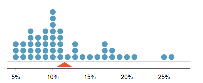
Think of a distribution: If you thought of a discrete one, let’s represent it in your head with a stacked dot plot. If it’s continuous, then think of a density plot. In either way, we would like to represent center of the distribution with a value that is around the most stacked (for the former) or most dense values (for the latter). So, we are looking for a value M that minimizes the expected distance between it and rest of the values of the distribution, in the long run (as a rule of thumb, always think in long runs when it’s a frequentist method). Most common way of defining the distance is squared difference which gets larger if two quantity is far away from each other: \((x - M)^2\). So, we need a value M that minimizes the following: \(\displaystyle \int p(x)(x-M)^2 \, dx\)
Guess which value minimizes the equation above? You probably guessed it right, since it’s also available from the preceding section: \(E[x]\). Here’s where things get very interesting for me. If you decide to go with \(|x - M|\) as the measure for distance, then it is the median that minimizes the expected distance in the long run. If you plug zeros for exact matches and ones for mismatches as a distance, you get the mode.
The beauty in mathematics or statistics is connection, at least to me. Even while writing this, I like how distances invoke vector norms, and minimization brings up calculus etc. This example connects mean, median, mode in my head, hence making it more intuitive. The book itself is great btw, if you’re interested in Bayesian methods I highly suggest it. Until next time, take care!